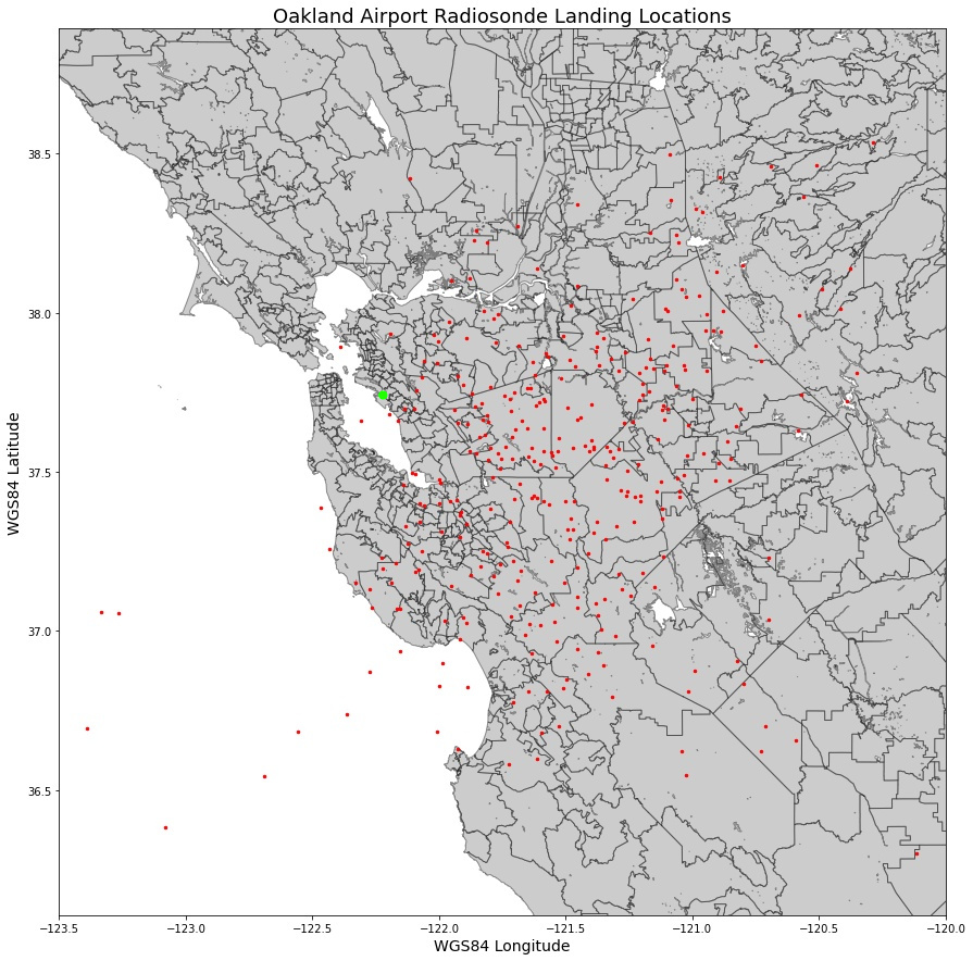
The prevailing winds here in California blow from west to east, from the Pacific Ocean towards the Sierra Nevada mountains. Radiosondes launched from Oakland International Airport float in these winds, landing east of Oakland in the Central Valley, or south in the hills east of San Jose. I never recover the ones that land in the Central Valley, as driving 2 hours each direction during rush hour to recover a balloon is a bit too far for me. Only rarely do they land in populated areas in the Bay Area, and almost never on the Peninsula or in the city of San Francisco.

This map (code below) shows the landing locations of all the radiosondes launched from Oakland since November 2020, when I started receiving them. Each red dot is the last position received by my two receiving stations, and is typically less than 1,000 meters altitude. This map shows 337 radiosondes, and I have removed the radiosondes launched up north by UCSD during atmospheric river events. As you can see, they are mostly south and east of the launch location (green dot).

When I saw the morning radiosonde on June 1st 2021 land just off the coast of Half Moon Bay, I thought the winds might be shifting favorably. I ran some predictions from Habhub, and those showed that the afternoon balloon might land in San Bruno, which is only 7 miles south of my apartment. The hunt was on!

My mobile receiving station is very simple, just a mag-mount antenna, RTL-SDR Blog v3, and laptop running Ubuntu. I use my phone's hotspot to view the Sondehub predicted landing location, and also upload decoded telemetry back to Sondehub. A navigator is useful to watch the screen and give directions.

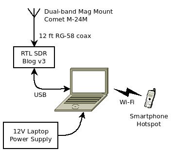
I use the radiosonde_auto_rx program to track the radiosondes, running entirely in a Docker container. Telemetry is automatically uploaded to Sondehub, so other people can watch the progress of the balloon. Sondehub also does a real-time prediction, updated as telemetry comes in, which is helpful when you are out in the field tracking the balloon. Radiosondes are launched twice daily at 1100 and 2300 UTC, and take about 90 minutes to ascend to 30,000 meters (~98,000 ft). Then the balloon bursts, and it takes only 30 minutes to fall back to the ground.

S4140428

This radiosonde was launched just after 2300 UTC on Tuesday June 1st 2021, which is 4pm Pacific time. It reached an altitude of 32,473 meters about 93 minutes after launch, and landed 20 minutes later.

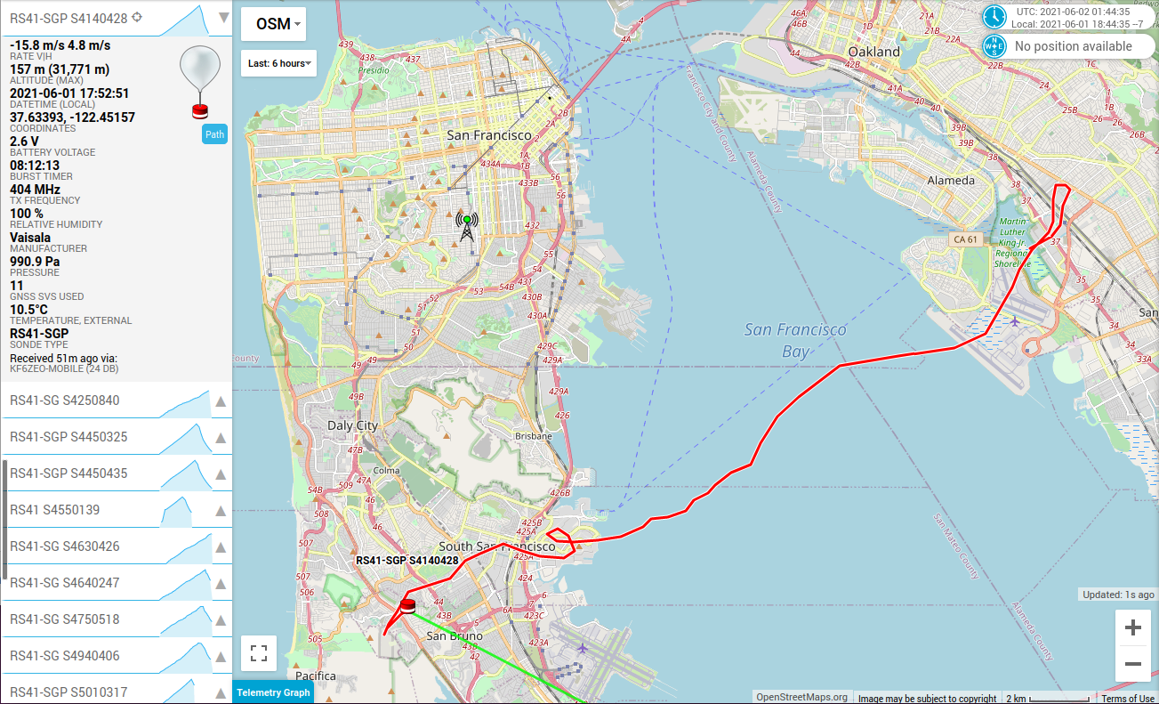
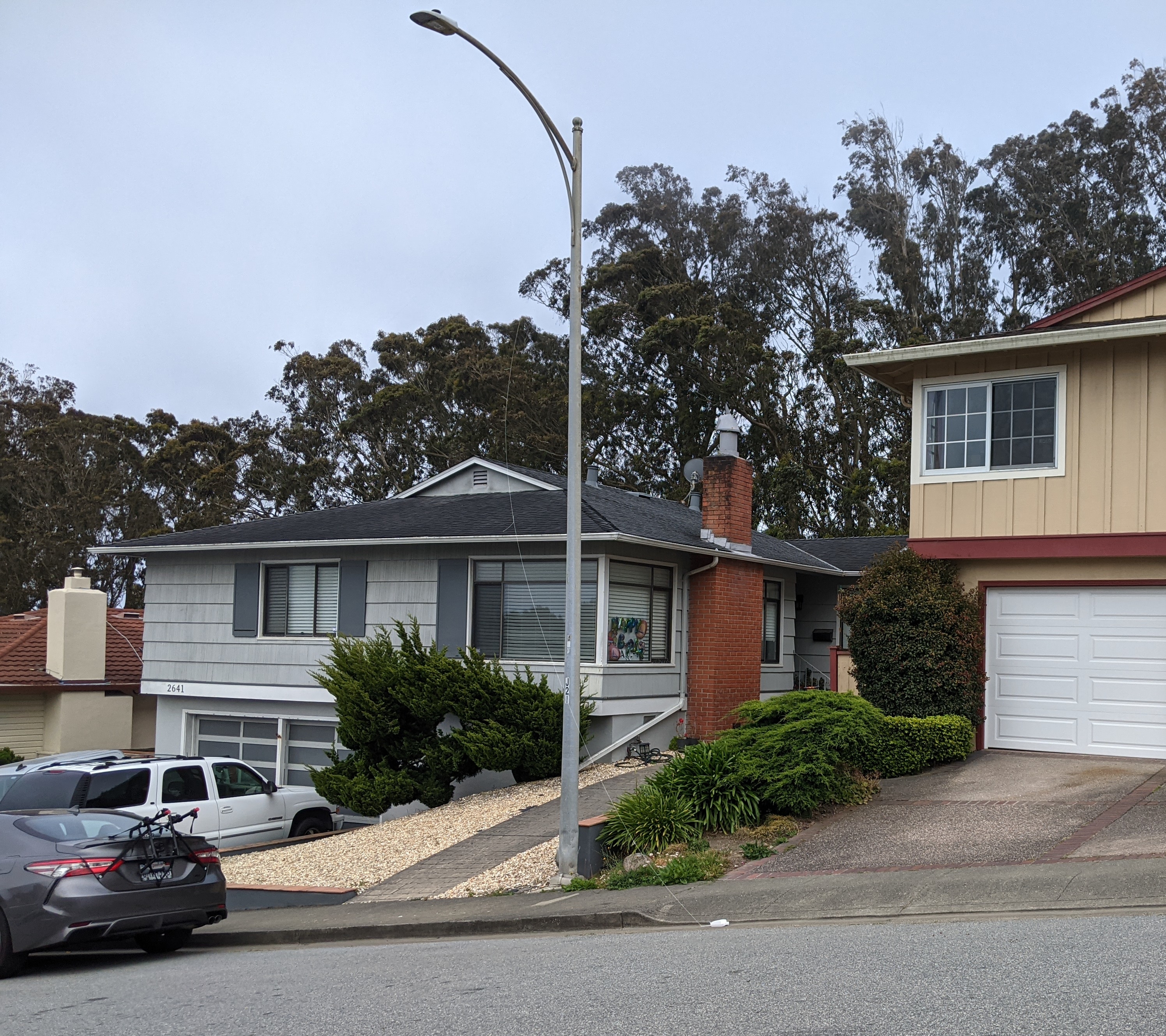
With my mobile station, I tracked it all the way to the ground and pulled up approximately 3 minutes after it landed. The tracker was in the street gutter, with the string draped over a streetlight and over a roof, and the actual balloon was hanging on the side of the house. I carefully pulled the balloon off the roof, cut the cable, and was gone before anybody knew what happened. Easy!

S4140438

The predictions for the Wednesday morning radiosonde had it landing in the middle of the bay, halfway between Oakland and San Francisco. Not much chance for a recovery I thought, so I didn't even set my alarm. Launch was at 1100 UTC on June 2nd 2021, which is 4am. But I woke up anyways at 6am, checked Sondehub, and saw that the balloon had just landed on Bernal Hill, only 0.9 miles from my house.

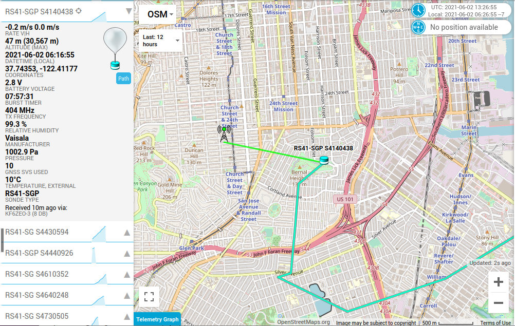
I jumped on my bike and was there in 25 minutes or so. The morning was very foggy and cool. The latex balloon was in the middle of Folsom St on the north side of the park, and the tracker electronics was behind a bush about 30 ft from the road. Thanks to all the road infrastructure we have built everywhere, recovery was very easy.

After getting back to the house, I took a look at the telemetry. I could see where the balloon had hit the ground at 1301 UTC, and slowly rolled (or got dragged by the balloon) down the hill over the course of 3 minutes, until signal was lost. When I picked the tracker up off the ground 28.5 minutes later, my station at home started receiving telemetry again.

On the bike ride home, I was treated to an amazing sunrise over our beautiful city.

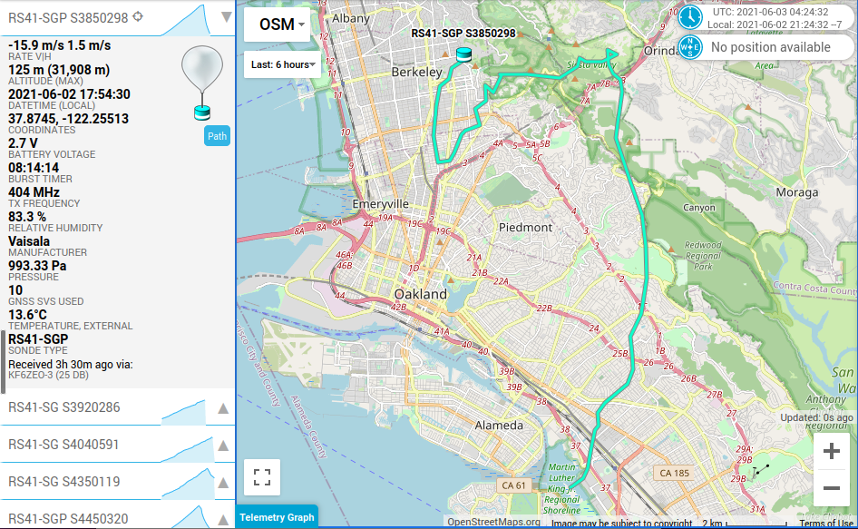
S3850298

The winds had shifted northerly for the 2300 UTC June 2nd 2021 launch, and the predictions had it landing in the hills east of Berkeley. I had meetings that evening, so I wasn't really paying attention. The radiosonde actually landed on the UC Berkeley campus, in the Stern Hall dorms only 300 feet northwest of the Greek Theatre. Hopefully some student was curious and grabbed it!

The winds have grown stronger, and the radiosondes are now landing in the Delta and Central Valley. Back to our regularly scheduled programming.

Code

The python3 code used to generate the plot at the top is based on earlier work plotting balloon locations. It basically grabs the last line (last decoded position, which is probably pretty close to the ground) of all the saved telemetry log files, and plots those on a map.

Jupyter notebook, using Jupyter 6.1.5, Python 3.8.5, Matplotlib 3.3.3, Pandas 1.1.5, and Geopandas 0.8.1.

Raw python3 code

Code, with the jupyter notebook comments:

#!/usr/bin/env python
# coding: utf-8

# In[1]:


import pandas as pd
import matplotlib.pyplot as plt
import descartes
import geopandas as gpd
import glob, os
import matplotlib as mpl
from shapely.geometry import Point, Polygon


# In[2]:


# Generate the census map diagram, and plot it
census_map = gpd.read_file('../TG00CAZCTA.shp')
census_map = census_map.to_crs('EPSG:4326')
fig,ax = plt.subplots(figsize = (15,15))
ax.set_ylim([37, 38.25])
ax.set_xlim([-122.75, -121.5])
census_map.plot(ax = ax, linewidth=1, edgecolor='black')


# In[3]:


# Make a list of all the log filenames in the folder.
all_files = glob.glob("*.log")

li = []

# Iterate thru each file and grab the last line. Append each last line to li list.
for filename in all_files:
    df = pd.read_csv(filename)
    df2 = df.tail(1)
    li.append(df2)

# Concat the list into a single dataframe.
dataframe = pd.concat(li, axis=0, ignore_index=True)

print(dataframe)


# In[4]:


# Create geometry points based on the lat/long from each row in the dataframe
geometry = [Point(xy) for xy in zip( dataframe["lon"], dataframe["lat"]) ]
dataframe[:3]


# In[5]:


# Make a GeoPandas dataframe from the dataframe and the geometry points
geo_frame = gpd.GeoDataFrame(dataframe,            #specify data
                             crs = 'EPSG:4326',    #specify coordinate ref system
                             geometry = geometry)  #specify geometry list created
geo_frame.head()


# In[6]:


# Plot the census map, then plot the GeoPandas dataframe on top.
fig,ax = plt.subplots(figsize = (15,15))
ax.set_box_aspect(1)
ax.set_ylim([37.0, 38.0])    # This doesn't do anything because aspect ratio is 1, set by longitude
ax.set_xlim([-123.5, -120.0])
ax.set_ylabel('WGS84 Latitude', fontsize=14)
ax.set_xlabel('WGS84 Longitude', fontsize=14)
ax.set_title('Oakland Airport Radiosonde Landing Locations', fontsize=18)

census_map.plot(ax = ax, alpha = 0.4, color="grey", linewidth=1, edgecolor='black')

geo_frame.plot(ax = ax, markersize = 6, color = "red", marker = "o")

# Save the plot locally
plt.savefig('last-position.jpg', bbox_inches='tight')


# In[ ]: